
Basics of Magnetic Resonance Imaging
Author
James G. Pipe, PhD
Division of Neuroradiology, Barrow Neurological Institute, St. Joseph’s Hospital and Medical Center, Phoenix, Arizona
Abstract
The field of magnetic resonance (MR) imaging has continued to benefit from technological advances since its introduction as a clinical tool. This article reviews the basic physics of MR imaging, discusses new imaging methods, and explores limitations to obtaining good images.
Key Words: echo time, gadolinium contrast enhancement, magnetic resonance imaging, proton density-weighted images, repetition time, T1-weighted images, T2-weighted images
Since its clinical introduction in the early 1980s, the impact of magnetic resonance (MR) imaging on diagnostic imaging has been enormous. The large variety of physical parameters that affect MR imaging creates a method rich with information and, often, with artifact. Maximizing the former while minimizing the latter is a continuing challenge for the MR imaging community. Significant advances in technology, from magnet design to contrast agent development to improvements in computer hardware and software, have fueled the development of this field. This article briefly reviews the physics underlying MR imaging and discusses some of the recent innovations that are advancing this field.
MR Imaging Signal
The production of electricity by a rotating magnet, a physical principle called Faraday’s law of induction, describes how an MR image signal is produced. Essentially, an MR scanner is an electrical generator with a computer that interprets the induced electrical currents to produce an image of in vivo magnetism. Creating an MR image therefore requires an in vivo magnetic source, a force (torque) that causes the magnetic source to rotate, and an appropriately placed coil of wire.
Magnetic Source
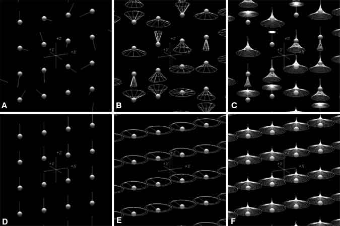
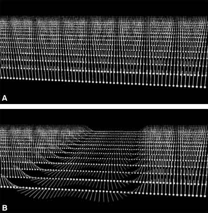
Organisms have magnetic sources in their bodies, located in the nuclei of atoms that compose water and organic molecules. These nuclear magnets, also referred to as spins, act similar to simple bar magnets with a north and south pole but have very weak forces and are oriented randomly (Fig. 1A).
When a patient is inserted into the tube of an MR imaging magnet, the magnetic field (called B0), which is quite strong, has two effects on individual spins. First, it causes them to precess about that magnetic field (Fig. 1B); second, it effectively lines up spins parallel to the direction of B0 (Fig. 1C and D). A confounding effect, however, is that slightly less than half of the spins actually line up in the opposite direction—antiparallel to B0—and cancel the magnetism of an equal number of parallel spins. About 10 of every million spins are detectable (parallel) in MR imaging; the remaining spins are split equally between parallel and antiparallel orientations. The combined magnetism from these few parallel spins creates a magnetic density that is still very weak, but strong enough for MR imaging as long as the spins remain aligned. For comparison, the strength of B0 is roughly 10,000 times stronger than the earth’s magnetic field, while a cubic centimeter of spins produces a magnetic field about 100,000 times weaker than the earth’s magnetic field. The complexity and expense of MR scanners reflect the need to produce the former field and to detect the latter.
Torque
After the spins are aligned parallel with B0, they are rotated perpendicular to B0. In this state, B0 produces a torque on the spins that causes them to precess rapidly at a frequency exactly proportional to the strength of B0, a rate called the Larmor frequency (Fig. 1E). For common clinical magnets with a B0 strength of 1.5 Tesla, the Larmor frequency is about 64 MHz, just below the frequency range on FM (frequency-modulated) radio.
The method for rotating the spins perpendicular to B0 involves the application of a rotating magnetic field, called a radio frequency (RF) pulse. This RF pulse is much weaker than B0 and must rotate at the same precessional frequency as the spins, or be in resonance, to have an effect. The process of rotating the spins into a signal-producing state is called excitation. After excitation, the spin immediately induces an electrical current in any nearby wires.
Coils
The coils of wire used for detection are called RF coils because they are designed to resonate at radio frequencies—specifically, at the Larmor frequency. A wide variety of RF coils can be used for signal detection. One example is the cylinder that slides over a patient’s head for a brain MR image. This device is composed of several smaller coils that act as one “supercoil”, called a quadrature coil. A similar but larger coil is embedded inside the tube of the magnet for general body imaging. Specialized coils are crafted for different applications so that they are as small as possible for any given part of the body. The coil should be compact and close to the area of interest because larger coils produce noisier images. Conversely, smaller coils can only detect signals from smaller regions.
Figure 2. T1, or longitudinal relaxation, describes the process of spin realignment with the applied magnetic field B0. T2, or transverse relaxation, describes the loss of the perpendicular precessing signal producing magnetization.
Features of the MR Signal
The strength of the current that is measured as the MR signal is directly related to the amount of spin magnetization precessing in the scanner. After the spins are excited by the RF pulse and begin precessing, several things happen that affect the MR signal (Fig. 2). The spins immediately begin to precess at a Larmor frequency exactly proportional to the local magnetic field strength. The spins realign themselves with the magnetic field B0 after a couple of seconds while the precessing magnetization (and the associated signal) fades in about 0.10 second. The second two processes are called relaxation and are characterized by the time constants T1 and T2, respectively. The different rates at which each process occurs reflect the local properties of each tissue, as discussed below.
Spin Realignment and Repetition Time
Field inhomogeneities that are much larger than spin motion cause reversible spin dephasing.
MR images take time to collect. Typically, spins must be excited many times, each time producing a slightly different measurement. The first relaxation mechanism, namely the longitudinal realignment of the excited spins with B0, must be allowed to occur (to some degree) between each excitation.
Otherwise, there is insufficient `realigned’ magnetization available for the excitations that follow and the resulting signal is diminished. The rate of this realignment is characterized by the time constant, T1, the time required for 63% of the complete magnetization to form after excitation. The ratio of the time between excitations (the repetition time, TR) and the T1 of spins in any given tissue indicates (but is not equal to) the relative fraction of signal that is produced if complete spin realignment is not allowed.
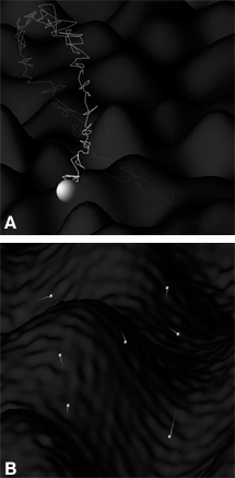
The cause of this spin realignment is known as spin-lattice relaxation. As nuclei oscillate and tumble in their molecular sea, they pass through locally changing magnetic fields (Fig. 3A). When a component of that motion is at the Larmor frequency through one of these changing magnetic fields, the nucleus `sees’ an effective resonant RF pulse that rotates it out of its current state. The collection of these randomly oriented RF pulses serves to speed the nuclear spin states toward their preferred alignment much like shaking a box of balls moves heavy balls to the bottom and light ones to the top.
Signal Loss and Echo Time
The realignment of spins toward a direction parallel to B0 naturally removes them from the plane transverse to B0, in which they precess to form the MR image signal. Therefore, the signal decays as the spins realign due to spin-lattice relaxation. An additional mechanism, however, dominates this transverse decay and can be explained by recalling that the frequency of spin precession is proportional to the local magnetic field. The molecular environment in which protons move has variations in the magnetic field (Fig. 3A). Thus, the precession of each spin is always speeding up and slowing down as it moves through these fields, slowly losing magnetic alignment with neighboring spins. This loss of spin coherence on a molecular scale is called spin-spin relaxation. The total loss of precessing (signal-producing) magnetization due to spin-lattice and spin-spin relaxation (the latter being the dominant mechanism) is characterized by the time constant T2, the time required for 63% of the precessing magnetization to decay.
The amount of signal decay depends on T2 and the time between the spin excitation and the measurement of the induced current in the coil, known as echo time (TE). As with the TR/T1 ratio, the TE/T2 ratio indicates the relative fraction of precessing magnetization (and therefore of the available signal) that remains at the time of measurement.
Large Scale Dephasing and Spin Echo
As excited spins move about the molecular landscape, the final phase angle that their magnetism is directed at the time of signal measurement reflects the average frequency at which they have precessed. In turn, this value reflects the average magnetic field strength to which they have been exposed. This magnetic field not only changes on a molecular scale (responsible for T1 and T2 relaxation), it also changes more slowly on a macroscopic scale (Fig. 3B). Thus, any region will have variations in the final phase of its spins, and its composite signal from all of these spins will be reduced. This signal loss is typically referred to as spin dephasing, and its rate, along with the less significant (in this context) mechanisms of spin-lattice and spin-spin relaxation, is characterized by the time constant T2*.
Although the loss of signal strength from T1 and T2 relaxation is unavoidable, the loss of signal from spin dephasing (T2*) can be reversed. The same applied resonant RF pulse that excited the spins can reverse the phase of all spins in the transverse plane. This 180º refocusing RF pulse puts the faster-precessing spins behind the slower ones. If 10 msec elapse after the initial spin excitation before this refocusing pulse is applied, the fast spins will catch up to the slow spins 10 msec after the refocusing pulse. Once again a coherent set of spins is created in what is called a spin echo. Data collection schemes with and without this refocusing pulse are called spin-echo and gradient-echo pulse sequences, respectively. The use of this rephasing is very important in regions of magnetic field inhomogeneity if TE is very long (Fig. 4). Rephasing works only if `fast’ spins remain fast before and after the refocusing pulse. These RF pulses do not refocus the dephasing that creates spin-spin (T2) relaxation, because it is caused by field changes on a molecular scale, and spins are speeding up and slowing down far too quickly to be refocused coherently.
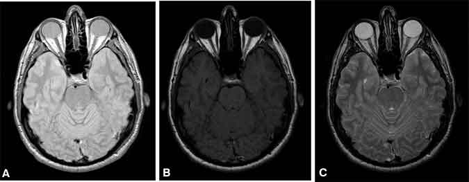
Image Contrast
Basic contrast in MR imaging relies on the differences in the density of water and fat, T1, and T2 of different tissues. The strongest signal is achieved with a long TR (allowing full spin realignment between excitations) and short TE (measuring the signal before significant T2 decay). Because the resulting image contrast is based mostly on the density of protons, such images are appropriately called proton density weighted (Fig. 5A). Beyond this, contrast is added only by making tissues darker. Adding image contrast based on differences in the T1 of tissues is achieved by reducing TR to a value about equal to the average T1 of the tissues of interest. Images with this modification are called T1-weighted images (Fig. 5B). This TR shortening preferentially darkens spins with longer T1 values, which do not recover as quickly as those with shorter T1 values. The addition of contrast based on differences in T2 is best achieved by measuring the MR image signal at a TE about equal to the average T2 of the tissues of interest, resulting in T2-weighted images (Fig. 5C).
This increase in TE preferentially darkens spins with shorter T2 values, which decay more rapidly than those with longer T2 values. T1 and T2 contrasts are rarely combined because objects that remain bright on a T1-weighted image tend to be dark on a T2-weighted image and vice versa. Thus, the combination of these weightings would result in an image where all tissues are dark—some from insufficient T1 recovery of spin alignment with B0, others from T2 decay of the precessing magnetization.
Contrast Agents
The endogenous spin-lattice (T1) and spin-spin (T2) relaxation mechanisms cannot be removed, but they can be increased by introducing exogenous agents that alter the local magnetic field. A common MR image contrast agent is a paramagnetic molecule containing a gadolinium atom with an unpaired electron, which has a magnetic field about 700 times greater than that of an individual proton spin. The added magnetic field inhomogeneity from such a contrast agent increases spin-lattice and spin-spin relaxation mechanisms, thereby decreasing the T1 and T2 of tissue that contains this agent. T1 shortening combined with a T1-weighted scan causes a brighter image while T2 shortening combined with a T2-weighted scan produces a darker image. Contrast agents have no effect on a truly proton density-weighted image. The relative amount of both spin-lattice and spin-spin relaxation depends on factors such as the shape and strength of the magnetic field produced by the agent, its concentration, its molecular size, and its affinity for water.
From Measured Electrical Current to Image
All methods of forming MR images rely on the application of magnetic field gradients. The appropriate placement of extra coils around an MR image scanner creates magnetic fields that vary linearly in any direction, by definition producing a spatial gradient in the magnetic field as well as the corresponding Larmor frequency of spin precession. The magnitude and direction of these field gradients can be changed in less than a millisecond. These field gradients are used to isolate the signal for image formation in two ways: slice selection and wave formation.
Slice selection is the limitation of spin excitation to a single plane. The excitation RF pulse contains a range of frequencies, approximately (but not limited to) 1000 Hz wide, that is centered around 64 MHz (for B0 = 1.5 Tesla). Because of the requirement for resonance, this pulse only excites spins precessing within that range of frequencies. When a field gradient is applied in a particular direction, the changing magnetic field in that direction creates a corresponding change in the Larmor frequency of precession. Only a limited range of spins in the direction of the applied field gradient will have Larmor frequencies corresponding to the frequency range of the RF pulse. The result is a plane of excitation orthogonal to the direction of the applied field gradient (Fig. 6). The plane can be translated by changing the frequency of the RF pulse and rotated by changing the direction of the field gradient.
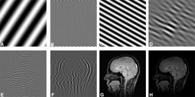
Once a plane of spins has been excited, the current induced in the RF coil is proportional to the magnetization from all the excited spins in the slice, which is measured as a single number. In contrast, the separate detectors in an array of detectors in digital radiography each simultaneously measures the signal at a single location in the imaging plane. In MR imaging a single detector (the RF coil) records consecutive measurements, each measurement providing information about the entire imaging plane. MR imaging takes advantage of the ability to separate any image into a series of waves, or spatial frequencies (Fig. 7).
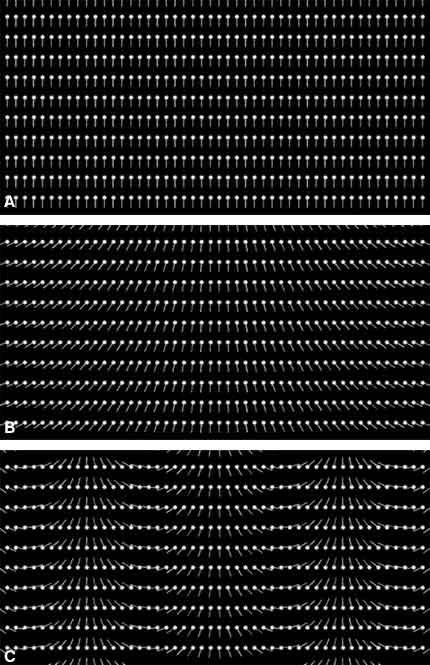
When a magnetic field gradient is turned on in a particular direction across an excited slice, spins on one side of the slice precess faster than those on the other side. A `twist’ of the spin phases is thereby formed across the image (Fig. 8). The longer the gradient field is on, the greater this twist becomes. The amount of twist can be characterized by the number of 360º cycles the phase turns across the prescribed field of view. If an excited plane of spins is defined by two directions x and y, the scanner is programmed to create many twists in the directions of both x and y after the spins are excited. Thus, each MR image signal measured corresponds to the amplitude of a particular (known) wave function across the entire image (Fig. 7). After a sufficient number of these waves have been measured, they are added together—weighted by the corresponding measured amplitude—to form the image. Mathematically, this summation of wave patterns is a Fourier transform .
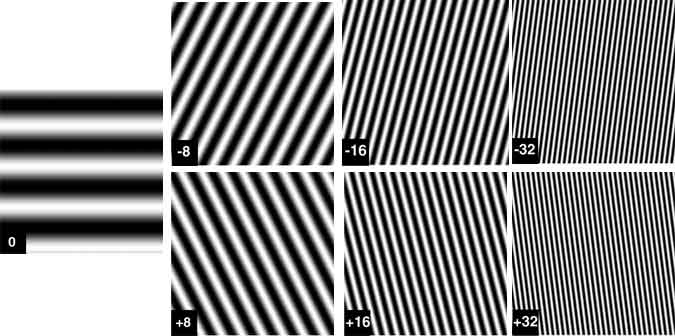
Typical image collection involves a series of measurements for each TR, in which some number of phase twists are induced in one direction (the phase-encoded direction). Data are measured as a magnetic field gradient is applied in the other in-plane direction, creating an evolving set of phase twists in that direction (the frequency-encoded direction; Fig. 9). For each TR the amount of phase twist in the phase-encoded direction is changed slightly, and the entire set of phase twists in the frequency-encoded direction is measured again. After a sufficient number of TRs, a `complete’ set of waves with phase twists in both the x and y directions is acquired. The matrix term associated with an MR image (e.g., 256 x 192) refers to the total number of waves measured in each direction.
An entity called k-space further describes how these different data, each corresponding to a particular wave, are collected. As measurements are collected, they are stored in a two-dimensional array in which the row and column of each measurement correspond to the amount of horizontal and vertical phase twists in the excited slice, respectively. This array, a k-space map of the collected data, can be considered an `image’ of the spatial frequencies contained in that slice and is a bookkeeping device used to relate each measured current value to the particular wave it represents (Fig. 10). The values in one row of k-space correspond to the series of measurements made during a single TR with increasing phase twists in the frequency-encoded direction. Individual rows correspond to the different amount of phase twists achieved in the phase-encoded direction.
New Methods in MR Imaging
The MR image signal depends on the interactions of intrinsic parameters such as the T1, T2, and T2* relaxation values and local magnetic field strengths with the operator’s choice of TE, TR, and the order of applying the RF pulses and magnetic field gradients. Consequently, images can be collected in innumerable ways, each producing a slightly different result. MR imaging becomes more like a soup in which different strategies can be added to obtain a particular flavor of image. Some of the new ingredients that have become available in the last few years are discussed below. The first three methods illustrate new ways to make image collection more efficient and robust; the last three methods indicate established ways of adding contrast that are becoming more practical in the clinical setting due to advances in technology.
Echo Planar Imaging
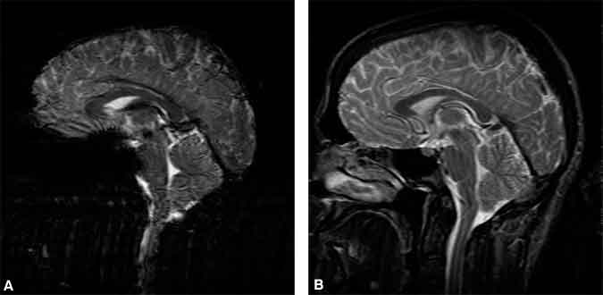
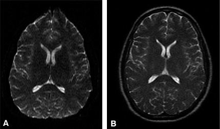
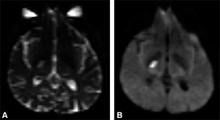
The T2 of many spins of interest ranges from 50 to 100 msec. In other words, after an excitation RF pulse, there is measurable (but decaying) signal for about 100 msec. In contrast, one set of frequency-encoded measurements (at one fixed phase encoding) can be collected in a few msec or less. If short imaging time is paramount, it is inefficient to measure the excited signal for a small fraction of the time that it is available. Rather than leaving the phase-encoding twist fixed during a readout while collecting only one complete set of frequency-encoding twists, the magnetic field gradient in the frequency-encoding gradient can be oscillated (producing the same complete set of twists multiple times). Concomitantly, the phase-encoding twist is altered slightly between each frequency-encoding gradient oscillation by a very small application of the phase-encoding field gradient. The entire set of waves (single-shot echo-planar imaging, EPI) or some subset of them (multi-shot EPI) can thereby be measured after a single excitation (in a single TR).[5] The advantage is that all of the available signal is used for image data collection. All the data for an EPI image (Fig. 11A) can be collected in less than 100 msec. A significant disadvantage of EPI is that the long duration of data collection can cause blurring (from T2-related amplitude decay) and geometrical warping (from spin phase accrual related to inhomogeneous magnetic fields).
Fast Spin Echo
The change in phase of spins during EPI data collection, which causes image warping, can be greatly reduced by applying 180º RF refocusing pulses (described above) multiple times during the middle of data acquisition. This strategy is less efficient than EPI because data cannot be collected during each RF pulse application. However, the improvement in the quality of a fast spin echo (FSE; Fig. 11B) is often worth the loss in efficiency.3 These RF pulses heat the patient like very inefficient bursts of microwave energy; thus, there is a limit to the number of refocusing pulses that can be applied in a given duration.

Spiral MR Imaging
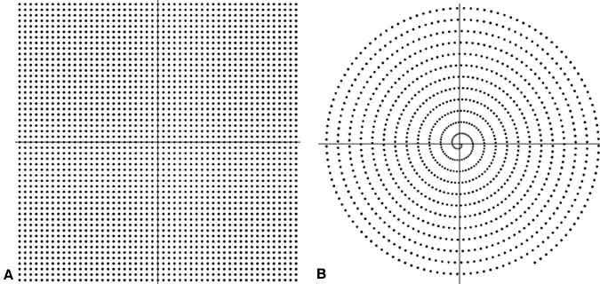
Conventional methods of data collection, along with the EPI and FSE methods described above, collect data with only the frequency-encoding field gradient on. Consequently, the spatial waves in a straight line through k -space (i.e., phase twists changing in one direction only) can be measured. The most notable reason is that image reconstruction with the Fourier transform is far more efficient when adding spatial waves measured in this fashion.
However, modern computational power combined with unconventional thinking has led to a myriad of data collection `pathways’ through k -space. One of the better known is a path that follows an Archimedean spiral.[1,6] By appropriately changing the direction and magnitude of the field gradient, data can be measured along a spiral path in k -space, which can be more efficient than conventional measurements on `linear’ paths (Fig. 12).
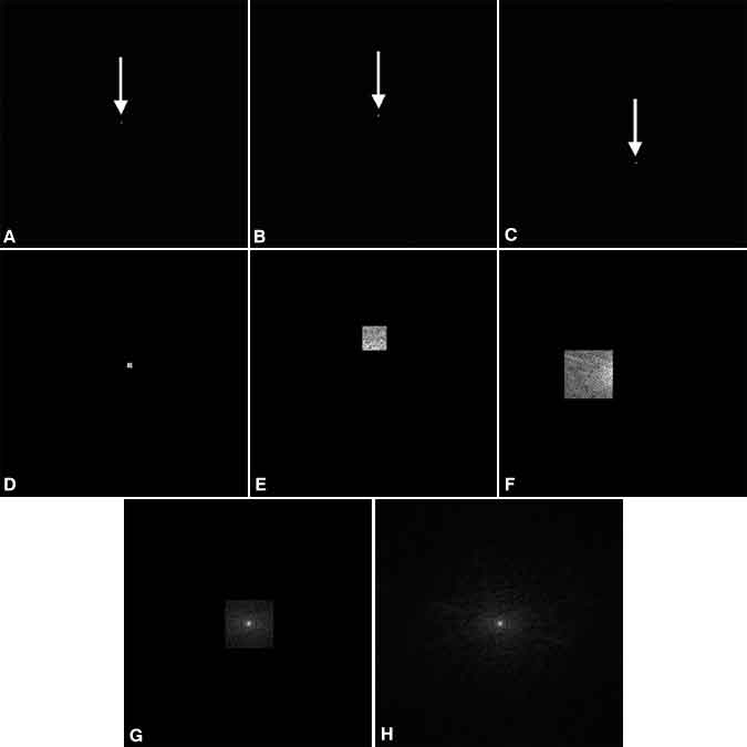
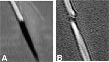
Importantly, the slowly varying waves—at the center of k-space—are measured first. These waves have the greatest effect on the final appearance of the image. Motion during the data measurement period, which can corrupt the image, only affects the measurement of rapidly varying waves collected later in the measurement. Spiral MR images are then much less prone to image artifacts from motion than conventional scans (Fig. 13).[7]
Diffusion-Weighted MR Imaging
The local magnetic field of spins varies so rapidly that they cannot be refocused, leading to spin-spin (T2) decay. This effect can be magnified significantly by applying strong magnetic field gradients for 20 to 80 msec before any data are measured. The effective `dephasing’ of the spins by random movement through this externally applied magnetic field is much greater than that of T2-decay mechanisms.[10] Because the change in the magnetic field is identical everywhere, the amount of added signal loss from dephasing is proportional only to the amount of diffusive motion of the spins while the applied gradient is on (Fig. 14).
Figure 15. Time course of a single pixel in the right motor cortex during activation studies, collected with a temporal resolution of one image/3 sec. The short horizontal line segments represent states of rest (lower set) and sequential finger tapping (upper set) that alternated every 15 sec.
Functional MR Imaging
The T2* dephasing effect is present in blood due to magnetic field disturbances from deoxyhemoglobin, which is paramagnetic. When data are collected at a long TE and without a refocusing RF pulse, the resulting image is very sensitive to magnetic field homogeneity, which is required for spins to stay aligned (have similar phases) as they precess. In these images the signal from blood and surrounding tissue is decreased with increased levels of deoxyhemoglobin. Luxury perfusion during neuronal metabolism creates an overly abundant supply of oxygenated blood flowing to activated tissue and a corresponding decreased level of deoxy-hemoglobin around the metabolizing neurons. By monitoring the strength of the MR image signal during motor or sensory tasks, the location of activated neuronal activity along with draining vascular beds can be inferred during these tasks. The difference in signal is small. Therefore, care must be taken to minimize signal fluctuations from other sources, such as bulk head motion and cardiac pulsations. This method is not sensitive to metabolism only, but rather to temporal changes in the difference between local oxygen supply and use (Fig. 15).
Figure 16. Temporal passage of a bolus of contrast agent with a pseudotemporal resolution of just under 2 sec/image from prebolus (upper left) to venous phase (lower right). These images are projections of a three-dimensional data set with 2-mm resolution in all directions. Although each entire data set took 20 sec to acquire, sophisticated data acquisition and reconstruction allow data to be shared between data sets to increase the perceived temporal resolution.
Contrast-Enhanced MR Angiography
The use of contrast agents in MR imaging is not new, but the use of contrast agents for MR angiography (CE-MRA) has incited considerable enthusiasm in the last few years due to advances in rapid scanning methods and technology. The physical key to its success is the dramatic shortening of intravascular T1 that can be achieved (from 1 second to about 15 msec). This increase in spin realignment with B0 allows the use of very short TRs (heavy T1 weighting). The effect on the signal from blood is minimal, and the signal from extravascular tissue is greatly reduced. Consequently, the image can be acquired rapidly: All data can be collected during the arterial phase of bolus passage (Fig. 16). Newer methods for data collection[4,8,11] also help increase imaging speed for targeting the arterial phase of bolus contrast.
Limits of MR Imaging
Many factors, such as obtaining the desired image contrast, reducing artifacts, reducing costs, and increasing patient acceptance, contribute to a “good” MR image. It is difficult to predict future trends for these factors, which are extremely variable and application dependent. Three factors of image quality, however, are well characterized: the signal-to-noise ratio (SNR), imaging time, and resolution. SNR is the ratio of the strength of the magnetism of precessing spins (MR image signal) relative to the random magnetic fields produced within the patient (noise). Resolution indicates the level of detail that can be seen in an image and is obtained by sampling wave patterns with a wavelength equal to the desired resolution distance (in all directions) as well as a complete set of waves that vary more slowly. The three quantities are related by the following equation:
SNR
a (voxel size)*(imaging time)1/2where the size of a voxel (short for volume element, the three-dimensional equivalent of a picture element, or pixel) is given by the product of the two in-plane resolutions multiplied by the slice thickness. For example, if an MR image is collected with in-plane resolution decreased from 1.0 mm2 to 0.5 mm2, SNR is reduced by a factor of four but can be restored by increasing imaging time sixteenfold.
The equation represents an unbreakable physical barrier. Technological barriers, however, lower the SNR from its optimal state for a given voxel size and imaging time and limit the minimum resolution and imaging time. These issues are addressed below, and some current and future solutions are considered.
Increasing SNR
A high SNR for a fixed voxel size and imaging time can be obtained by increasing in vivo magnetization or the efficiency of detection. Magnetization can be increased by increasing the magnetic field B0 in which the patient is being scanned. The fraction of parallel, or detectable spins (roughly 10/million), is proportional to B0. Doubling the magnet strength of a scanner doubles this fraction and doubles the MR imaging signal to a first approximation. Higher manufacturing costs, patient safety, and other field strength-related phenomena are hindrances to using higher field strengths, but the simple notion that doubling the SNR can reduce scan time by a factor of four (from the above equation) for many scans is a powerful motivator.
The efficiency of detection can be increased by the proper choice of RF coils. Small coils are less noisy than large ones, but they can only detect signal from a limited area. Recent advances have led to phased array coils,[9] sets of coils that act independently but together measure signal from a wide area. Signal detection with a large set of small coils is typically less noisy than that obtained with one large coil. The drawback of phased array coils is the added hardware and computer power necessary to process multiple signals.
Imaging Time
Imaging time is limited by how fast all the spatial waves in k-space necessary to complete an image with the desired resolution can be collected. These waves are produced by turning on the field gradients. Stronger field gradients can produce a greater variety of waves in a shorter amount of time than can weaker field gradients. To measure a two-dimensional set of waves, these gradients must be able to change direction rapidly so that the signal can be sampled over all of k-space. Thus, larger gradient amplitudes and gradients with higher slew rates (the rate at which the gradient can change direction) allow data to be collected more rapidly. Smarter sampling strategies (e.g., sampling trajectories through k-space) also help reduce imaging time. A recent advance is `real-time’ MR imaging. Still in its infancy, this technique includes real-time tracking of interventional devices, interactive movement of the imaging plane, and monitoring the passage of a bolus of contrast agent.
At least two factors involving patient safety may ultimately impose lower limits on imaging time: the specific absorption rate (SAR) and field gradient-induced nerve stimulation. The first factor, SAR, relates to patients becoming heated from exposure to the RF pulses. The RF pulses stimulate charged matter to vibrate at the Larmor frequency and add thermal energy to the patient. Current guidelines from the Food and Drug Administration limit power deposition to an amount which, if the patient had absolutely no cooling mechanisms at all, would heat the patient about 1º C/hour. Consequently, the amount of RF that can be used to excite and refocus spins is limited. The second factor, nerve stimulation, occurs when the field gradients are switched too rapidly, inducing current flow in the affected nerves. Although many have experienced peripheral nerve stimulation, which is probably harmless, ventricular fibrillation must not be induced. Proper design of the coils that create field gradients can minimize, but not eliminate, this effect.
Resolution
Other than limited SNR, which is a significant limitation to high-resolution MR images, other barriers are surmountable. Higher resolution scans require more computer memory and faster computer processing. A set of 128 slices, each producing a 512 x 512 pixel image and sampled from a four-element phased array coil set, requires about a gigabyte of memory. This is now possible but was less feasible just 5 years ago. Component stability, necessary for precise spatial encoding, is also improving through the use of shielded gradient coils, an innovation that is critical to obtaining advanced sequences such as EPI and spiral scanning.
Another barrier to improved resolution is physiologic motion from bulk motion, peristalsis, respiratory motion, and cardiac motion. The different time scales of these motions present different challenges for collecting data. Physiological motion can be circumvented in three ways. First, the motion can be monitored and the imaging data collected only during a quiescent period when tissues are assumed to return to the same state. Second, the motion can be monitored and corrected when the image is reconstructed. Finally, the image data can be collected fast enough to avoid the motion. The first scheme has been the basic way to obtain routine images in the abdomen, with the use of cardiac and respiratory gating. An effective application of the second scheme is the use of navigator echoes[2] in cardiac examinations to correct for respiratory motion. The third scheme is the most robust because motion can often be too unrepeatable and too complex for the first two schemes. Again, however, high-resolution scans collected in a brief time have a limited SNR.
Summary
The MR image signal represents the coherent magnetization of atomic nuclei, called spins, within the patient. This magnetization is perturbed, or excited, to a state in which it induces current in receiver coils. Afterward, it decays quickly with a time constant T2 and regrows more slowly with a time constant T1. The ratio of the time TE between each excitation and the corresponding current measurement and the tissue T2 value, as well as the ratio of the time TR between subsequent excitations and the tissue T1 value, largely determine the signal strength for a particular tissue. Nonuniformity in the magnetic field can cause additional incoherence in the signal within a voxel, leading to a more rapid decay of the signal for a gradient-echo image. This dephasing can be reversed by a refocusing RF pulse, which is used for spin-echo imaging.
Magnetic field gradients permit linear changes in the magnetic field and allow the selective excitation of a plane of spins. Application of varying magnetic field gradients after excitation creates evolving phase twists in the plane of spins. The resulting individual measurements of spatial waves are summed after data collection to form the image. The manner in which these waves are collected trades off various measures of image quality and total data collection time. New methods, however, continue to improve these tradeoffs.
The quality of the MR images is limited by a fundamental relationship between voxel size (resolution), image noise, and imaging time. None of these factors can be reduced without increasing one of the other two. The use of magnetic fields higher than 1.5 Tesla and further refinements of receiver coils will reduce image noise, which can be traded off for reduced imaging time or better resolution. Improvements in hardware will continue to reduce imaging time when voxel size and noise are sufficiently small.
References
- Ahn CB, Kim HH, Cho ZH: High-speed spiral-scan echo planar NMR imaging. IEEE Trans Med Imag MI-5:2-5, 1986
- Ehman RL, Felmlee JP: Adaptive technique for high-definition MR imaging of moving structures. Radiology 173:255-263, 1989
- Hennig J, Nauerth A, Friedburg H: RARE imaging: A fast imaging method for clinical MR. Magn Reson Med 3:823-833, 1986
- Korosec FR, Frayne R, Grist TM, et al: Time-resolved contrast-enhanced 3D MR angiography. Magn Reson Med 36:345-351, 1996
- Stehling MK, Turner R, Mansfield P: Echo-planar imaging: Magnetic resonance imaging in a fraction of a second. Science 254:43-50, 1991
- Meyer CH, Hu BS, Nishimura DG, et al: Fast spiral coronary artery imaging. Magn Reson Med 28:202-213, 1992
- Nishimura DG, Irarrazabal P, Meyer CH: A velocity k-space analysis of flow effects in echo-planar and spiral imaging. Magn Reson Med 33:549-556, 1995
- Pipe JG: Rapid contrast-enhanced MRA with PROPELLER MRI. Proceedings of the 7th Scientific Meeting of the International Society of Magnetic Resonance in Medicine 157, 1999
- Roemer PB, Edelstein WA, Hayes CE, et al: The NMR phased array. Magn Reson Med 16:192-225, 1990
- Stejskal EO, Tanner JE: Spin diffusion measurements: Spin echoes in the presence of a time-dependent field gradient. J Chem Phys 42:288-292, 1965
- Wilman AH, Riederer SJ, Huston J 3d, et al: Arterial phase carotid and vertebral artery imaging in 3D contrast-enhanced MR angiography by combining fluoroscopic triggering with an elliptical eccentric acquisition order. Magn Reson Med 40:24-35, 1998